---
title: "Simulation of Realized Infection Risk"
description: "simulate a probability distribution of risk"
author:
- name: Kayla Kauffman
url: https://https://kmkauffm.github.io/
orcid: 0000-0002-4897-9428
format:
html:
toc: true
toc-location: left
message: false
warning: false
code-fold: true
code-tools: true
theme: sandstone
bibliography: references.bib
date: 2023-12-15
categories: [R, code, simulations] # self-defined categories
image: schema.png
draft: false # setting this to `true` will prevent your post from appearing on your listing page until you're ready!
---
```{r}
#| echo: false
#| message: false
# library(spDataLarge)
library(tidyverse)
library(sf)
library(terra)
library(SiMRiv)
library(patchwork)
theme_set(theme_bw())
theme_update(plot.title = element_text(hjust = 0.5),
plot.subtitle = element_text(hjust = 0.5))
```
# Introduction
My research broadly addresses how land use change impact zoonotic disease sharing patterns between wildlife, domestic animals and people. One aspect of this research delves into how well a landscape of risk [@weinstein2018] can be predicted across space and time [@albery2022], and if people that spend more time in areas of high pathogen prevalence on the landscape are more likely to be infected with that parasite. The landscape of risk is the variation in pathogen density or pressure across the landscape, and the underlying environmental characteristics that permit pathogen persistence and onward transmission to susceptible individuals visiting that area (e.g., [@titcomb2021]).
Prior to doing this with actual data I want to set up a simulation so I can figure out some of the methods using a simplified scenario. In particular I am interested in comparing how noise in the dataset due to the variability in individuals home range sizes and susceptibility to infection affect my ability to associate cumulative exposure risk to infection probability. For my purposes here susceptibility encompasses variability in behavior of individuals that influence pathogen exposure, immunological function, genetics, etc [@sweeny2022].
# Risk Map
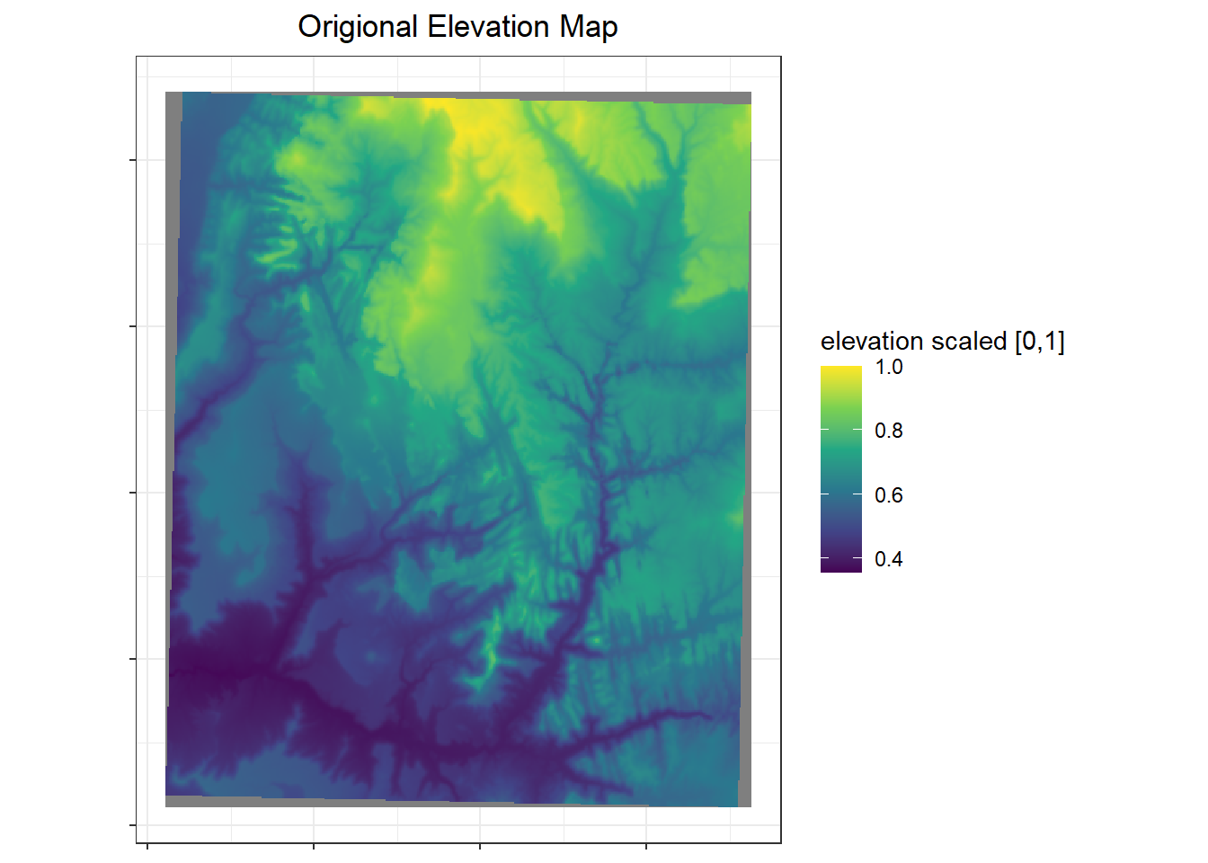
I am using the elevation raster of Zion National Park included in the `spDataLarge` package as the landscape risk map. The thought behind using this and not simply a simulated raster is to have highly variable patterns and spatial autocorrelation. However to use this, I need the values to fall between 0 and 1. This is what the original maps looks like with the scaled values.
```{r}
## load the data from the spDataLarge package
riskmap <- rast(system.file("raster/srtm.tif", package = "spDataLarge"))

## project in utm so easier units for making the simulated tracks
riskmap <- project(riskmap, "EPSG:26912")

## make values [0,1]
riskmap <- riskmap/max(values(riskmap), na.rm=T)

## most places should be pretty low
## look at the 'original values'
ggplot() +
  stars::geom_stars(data = stars::st_as_stars(riskmap)) +
  scale_fill_viridis_c() +
  coord_fixed() +
  labs(x=NULL, y=NULL, fill = "elevation scaled [0,1]", title = "Origional Elevation Map") +
  theme(axis.text = element_blank()) # since don't care about location
```
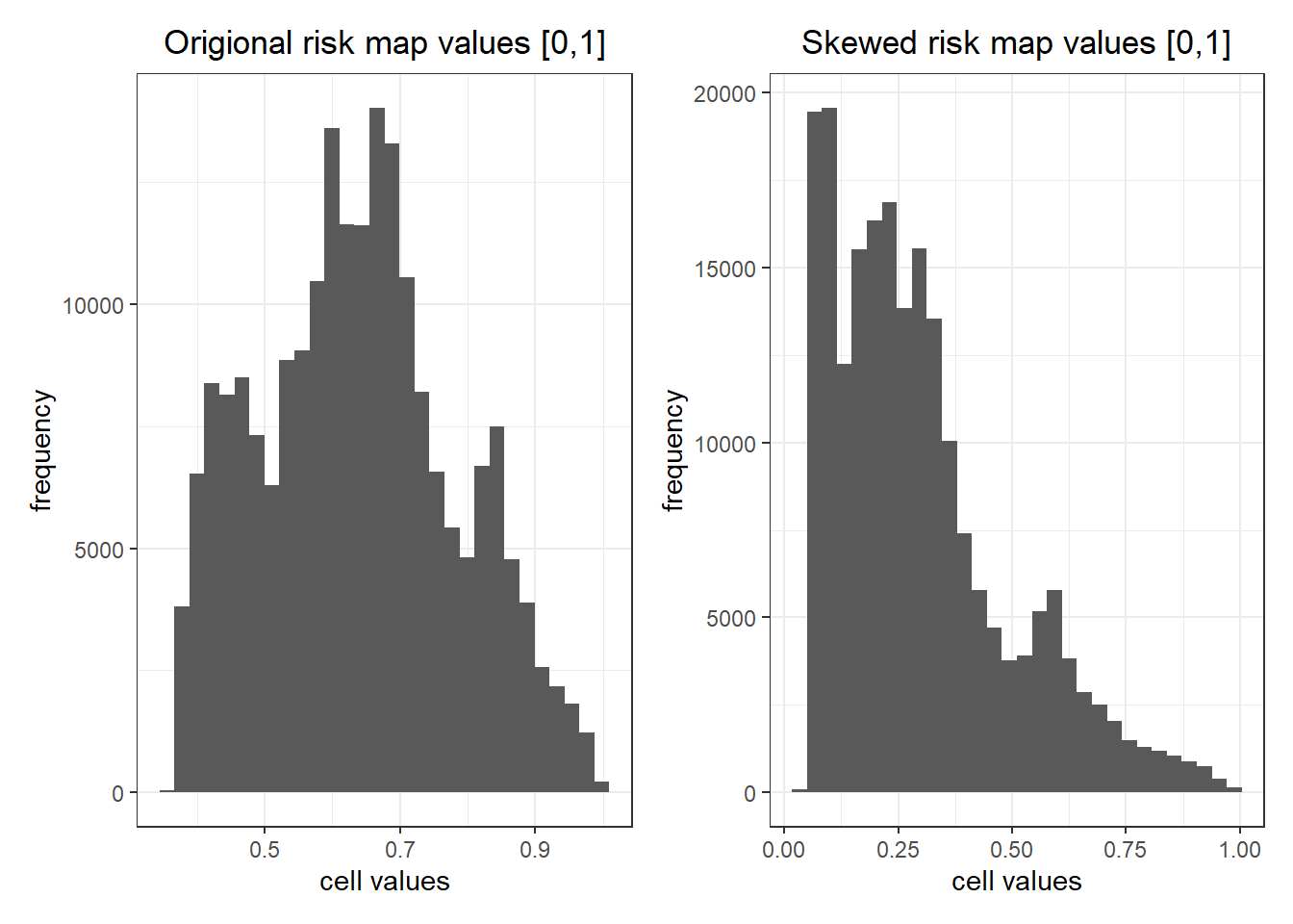
I want the values to be right skewed so that most places are low risk. So I transformed the values to values^3^ in my scaled raster to get the desired distribution of risk (pathogen density) in my risk map.
```{r}
## histogram of value distribution
p1 <- values(riskmap) %>%
  as.data.frame() %>%
  filter(is.finite(srtm)) %>%
  ggplot() +
  geom_histogram(aes(x=srtm)) +
  labs(x = "cell values", y = "frequency", title = "Origional risk map values [0,1]")

## add right skew to values so most are low
riskmap <- riskmap^3

## plots to commpare old and new value distributions
p2 <- values(riskmap) %>%
  as.data.frame() %>%
  ggplot() +
  geom_histogram(aes(x=srtm)) +
  labs(x = "cell values", y = "frequency", title = "Skewed risk map values [0,1]")

## plot old and new next to each other
p1+p2
```
```{r}
#| include: false
rm(p1, p2)
```
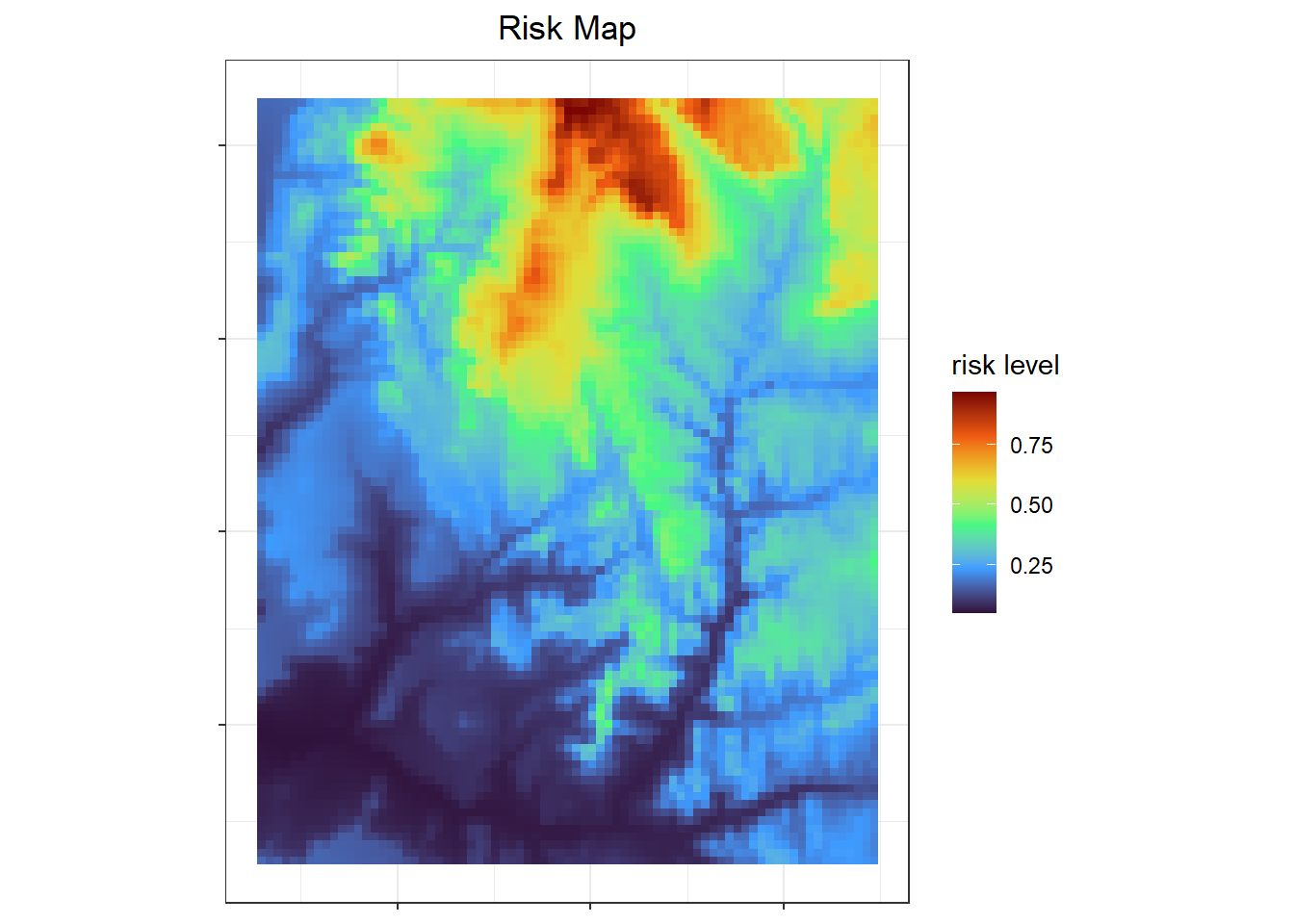
To make things run quickly, I aggregated the risk map so the resolution is lower. Then cropped the map to a squarer area so individuals don't fall outside of the area with values (the grey parts of the map above).
```{r}
## make resolution lower so things run quickly
riskmap <- aggregate(riskmap, fact=5, fun="mean")

## make square
tmp <- vect(ext(riskmap)-1500, crs=crs(riskmap))
riskmap <- crop(riskmap, tmp)

## plot the new lower resolution map
ggplot() +
  stars::geom_stars(data = stars::st_as_stars(riskmap)) +
  scale_fill_viridis_c(option = "H") +
  coord_fixed() +
  labs(x=NULL, y=NULL, fill = "risk level", title = "Risk Map") +
  theme(axis.text = element_blank()) # since don't care about location
## check the data structure
# riskmap
```
```{r}
#| include: false
rm(tmp)
```
# Single simulation
I am using a single simulation to figure out how to set up the simulation and to outline the process involved in the simulation. Once that is ironed out, I'll put everything into a single function so I can repeat the simulation many times and get confidence intervals for my estimated effects.
## Simulate movement
To simulate movement of individuals I followed the [`SiMRiv` vignette](https://cran.r-project.org/web/packages/SiMRiv/vignettes/SiMRiv.pdf). I wanted to have two types of movement to use in my simulation. I am calling these:
- **Simple random walk** - Single-state uncorrelated movement in an homogeneous landscape using Brownian motion [@turchin1998] to make individuals 'vibrate' in place. Movement of only this type is the 'null' state because an individual essentially staying in one place will have an exposure risk equal to their singular location. This state will be used to demonstrate that an individual's probability of infection is proportional to their exposures.\
- **Complex correlated walk** - Multistate correlated movement in a heterogeneous landscape using Levy walk-like movement with two-state movements composed of small random walks and bursts of longer correlated random walks [@reynolds2010]. A heterogeneous landscape is used to makes some areas high resistance, thus the population's movements will look more similar, since most movement will follow low resistance 'paths' (roads), but individuals will still randomly branch off into higher resistance areas.
An important part of simulating movement is the step length, which need to be relevant to the animal and the resolution of the raster. To limit movement in the simple random walk, make step sizes 1/20th of the resolution of the risk map. Find the resolution of the risk map. The resolution show help with choosing a step length that is relative to the pixel sizes so that individuals can move, but not too much within a given step. Steps of \~1/10 a pixel seem reasonable.
```{r}
## save cell size
cell_size = res(riskmap)[1]

## number of steps
nsteps = 1000

## random walk with step lengths relative to rast resolution
rand.walk <- state(concentration = 0, #turning angle concentration; 0=random
                             pwind = perceptualRange("gaussian", # centered on indiv's position
                                                     cell_size/5), ## radius of perceptual range 1/4 of steplength
                             steplen = cell_size/20, #maximum step length
                             name = "tight_random") #name of the state

## correlated walk with step lengths relative to rast resolutions
corr.walk <- state(concentration = 0.9, #turning angle concentration; 1=straight line
                             pwind = perceptualRange("circular", # gives equal weight to all pixels centered on current position
                                                     cell_size*2), ## radius of perceptual range 1/4 of steplength
                             steplen = cell_size/5, #maximum step length
                             name = "correlated") #name of the state

## using those states make walkers
rand.walker <- species(states = rand.walk)
## set up levy walker walk
levy.walker <- species(states = c(rand.walk,
                                  corr.walk),
                       trans = transitionMatrix(0.05, 0.01)) #probabilities of changing state 1 -> 2 and 2 -> 1
```
### Simple random walk
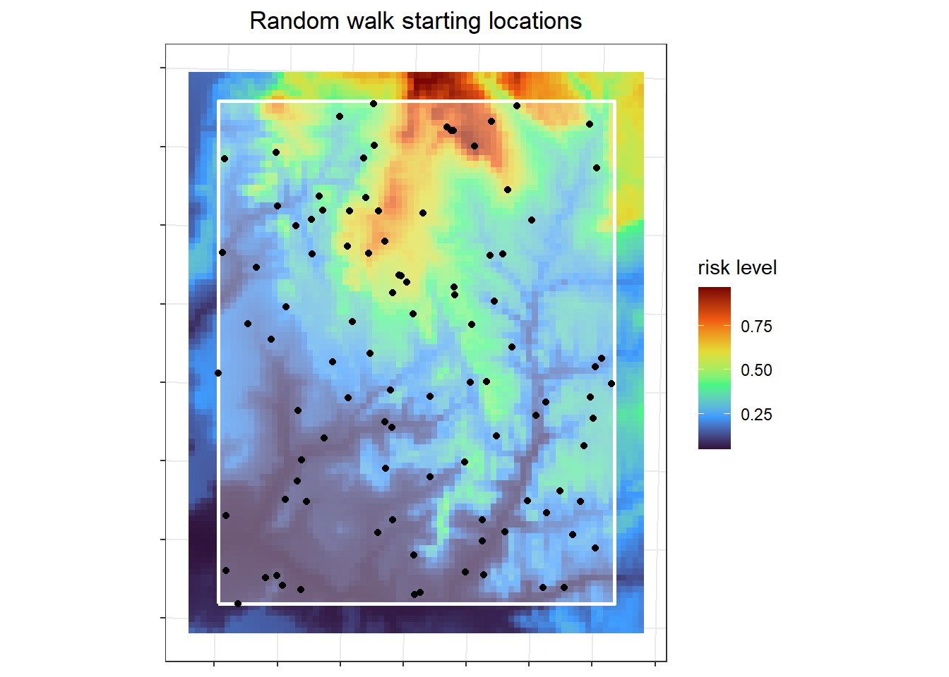
I simulated the simple random walks for 100 individuals all starting at randomly selected areas with in an area of interest (aoi). Because individuals can run off the edge of the raster, the starting locations should not be near the edge. The area of interest is the white rectangle, with each point representing an individual's starting location.
```{r}
#| message: false
#| warning: false
## generate random starting points
### avoid edges by defining area of interest more inside the risk map
### find bounding box of risk map
aoi <- st_bbox(riskmap)
### make insto sfc (spatial) object
aoi <- st_as_sfc(aoi)
### buffer to be 5 cells from edge of riskmap
aoi <- st_buffer(aoi, -cell_size*5)

# aoi <- crop(riskmap, aoi)
# ggplot() +
#   stars::geom_stars(data = stars::st_as_stars(riskmap)) +
#   scale_fill_viridis_c(option = "H") +
#   coord_fixed() +
#   labs(x=NULL, y=NULL, fill = "risk level", title = "Area of interest for starting locations on Risk Map") +
#   theme(axis.text = element_blank()) +# since don't care about location
#   geom_sf(data = aoi, fill = "white", alpha = 0.3, color = "white", lwd = 1)

start_coord <- st_sample(aoi, 100, type = "random")

## plot it
ggplot() +
  stars::geom_stars(data = stars::st_as_stars(riskmap)) +
  scale_fill_viridis_c(option = "H") +
  coord_fixed() +
  labs(x=NULL, y=NULL, fill = "risk level", title = "Random walk starting locations") +
  theme(axis.text = element_blank()) +# since don't care about location
  geom_sf(data = aoi, fill = "white", alpha = 0.3, color = "white", lwd = 1) +
  geom_sf(data = start_coord)
```
The random walks for all the individuals look like my intended "vibrating in place" outcome, such that individuals will spend all their time in just a few pixels, so theoretically their exposure risk is less variable.
```{r}
#| message: false
#| warning: false
## need the locations as a nx2 matrix
# start_coord_mat <- as.matrix(as.data.frame(start_coord, geom="xy"))
start_coord_mat <- st_coordinates(start_coord)

## simulate single state walks of 1000 steps
sim.rw <- list()
for (i in 1:100) {
  ## simulate from location i
  tmp <- simulate(rand.walker, nsteps,
                   coords = start_coord_mat[i,])
  ## save results to a list
  sim.rw[[i]] <- cbind(tmp[,1], tmp[,2])
}

## make in to sfc lines
sim.rw.sfc <- lapply(sim.rw, st_linestring)
sim.rw.sfc <- st_sf(id = 1:100, geometry = sim.rw.sfc) %>%
  st_set_crs(st_crs(riskmap))

## plot it
ggplot() +
  stars::geom_stars(data = stars::st_as_stars(riskmap)) +
  scale_fill_viridis_c(option = "H") +
  coord_fixed() +
  labs(x=NULL, y=NULL, fill = "risk level", title = "Random walks") +
  theme(axis.text = element_blank()) +# since don't care about location
  geom_sf(data = sim.rw.sfc)
```
```{r}
#| include: false
## clean up
rm(start_coord, sim.rw)
```
### Correlated walks
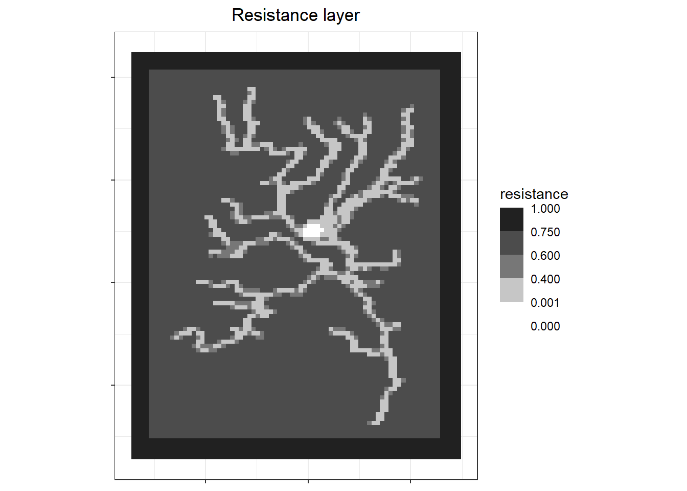
A resistance raster is needed to get correlated (levy walker) walks that are similar between individuals.
```{r}
#| message: false
## basemaps for resistance --NOT using because individual end up in a hairball
# landcover <- resistanceFromShape(
# system.file("doc/landcover.shp", package="SiMRiv")
# , res = 50, field = "coverclass", mapvalues = c(
# "forest" = 0.5, "urban" = 1, "dam" = 0
# , "shrubland" = 0.75), background = 0.95)
#
## river shape is the main resistance, because walks will follow paths
river.shape <- sf::st_read(system.file("doc/river-sample.shp", package="SiMRiv"), quiet = T)

## resistence surface
resistance <- resistanceFromShape(river.shape, #system.file("doc/river-sample.shp", package="SiMRiv"),
                                       # baseRaster = landcover, ## not using
                                  res =50, #provide when don't provide basemap
                                       buffer = 300, field = 0.01,
                                       background = 0.75, margin = 3000)

## add central area with low resistence so individuals start in roughly the same place
river.cent <- st_buffer(st_centroid(st_union(river.shape)), 200)
resistance <- resistanceFromShape(river.cent,
                                  baseRaster = resistance,
                                  buffer = 1000, field = 0,
                                  background = 1, margin = 3000)
# buffer here is just some magical function to convert river
# order into a meaningful value in the [0, 1] range!
# plot(resistance, axes = F, main="resistence raster")
# resistance
```
```{r}
#| include: false
rm(river.shape, river.cent)
```
Then the resistance raster should be down sampled and moved to the same location as the risk map.
```{r}
## move the resistence 'rivers' to the same location as the risk map
resistance <- rast(nrows = dim(resistance)[1],
                   ncols = dim(resistance)[2],
                   nlyrs = 1,
                   names = "resistance",
                   extent = st_bbox(aoi),
                   vals = values(resistance),
                   crs = crs(riskmap))

## resample to resolution matches riskmap
resistance <- resample(resistance, riskmap, method = "rms")

## make NAs to 1
resistance[is.na(resistance)] = 1

## plot it
ggplot() +
  stars::geom_stars(data = stars::st_as_stars(resistance)) +
  scale_fill_steps(breaks = c(0, 0.001, 0.4, 0.6, 0.75, 1),
                   low="white", high = "black") +
  # scale_fill_viridis_c(option = "H") +
  coord_fixed() +
  labs(x=NULL, y=NULL, fill = "resistance", title = "Resistance layer") +
  theme(axis.text = element_blank()) # since don't care about location
```
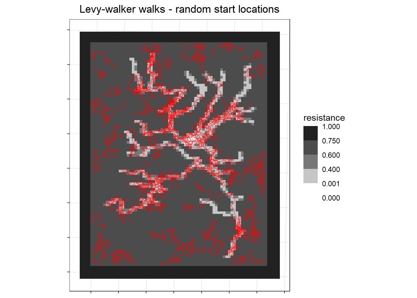
At first I tried using the same random starting locations as above to generate my correlated walks for each individual.
```{r}
#| message: false
#| warning: false
## simulate single state walks of 1000 steps
sim.rw <- list()
for (i in 1:100) {
  ## simulate from location i
  tmp <- simulate(levy.walker, nsteps,
                  resist = raster(resistance),
                   coords = start_coord_mat[i,])
  ## save results to a list
  sim.rw[[i]] <- cbind(tmp[,1], tmp[,2])
}

## make in to sfc lines
sim.rw.bad <- lapply(sim.rw, st_linestring)
sim.rw.bad <- st_sf(id = 1:100, geometry = sim.rw.bad) %>%
  st_set_crs(st_crs(riskmap))

## plot it
ggplot() +
  stars::geom_stars(data = stars::st_as_stars(resistance)) +
  scale_fill_steps(breaks = c(0, 0.001, 0.4, 0.6, 0.75, 1),
                   low="white", high = "black") +
  # scale_fill_viridis_c(option = "H") +
  coord_fixed() +
  labs(x=NULL, y=NULL, fill = "resistance", title = "Levy-walker walks - random start locations") +
  theme(axis.text = element_blank()) +# since don't care about location
  geom_sf(data = sim.rw.bad, col="red", alpha=0.5)
```
```{r}
#| include: false
rm(sim.rw, tmp, sim.rw.bad, start_coord_mat)
```
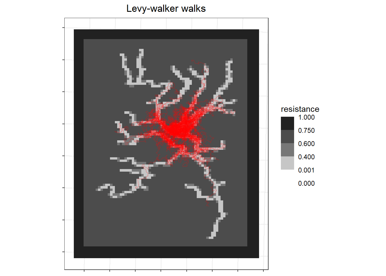
However, to make this more realistic, my correlated walks should also act like individuals following paths then delving off into different areas such as people accessing their crop fields. So instead of using random starting locations, I made the starting locations only be in low resistance areas.
```{r}
#| message: false
#| warning: false
## new starting coords in areas of low resistance so don't get stuck
init = xyFromCell(resistance, sample(which(values(resistance) == 0), 100, replace=T))

## simulate
sim.rw <- list()
for (i in 1:100) {
  ## simulate from location i
  tmp <- simulate(levy.walker, nsteps,
                  resist = raster(resistance),
                   coords = init[i,])
  ## save results to a list
  sim.rw[[i]] <- cbind(tmp[,1], tmp[,2])
}

## make in to sfc lines
sim.rw.levy <- lapply(sim.rw, st_linestring)
sim.rw.levy <- st_sf(id = 1:100, geometry = sim.rw.levy) %>%
  st_set_crs(st_crs(riskmap))

## plot it
ggplot() +
  stars::geom_stars(data = stars::st_as_stars(resistance)) +
  scale_fill_steps(breaks = c(0, 0.001, 0.4, 0.6, 0.75, 1),
                   low="white", high = "black") +
  # scale_fill_viridis_c(option = "H") +
  coord_fixed() +
  labs(x=NULL, y=NULL, fill = "resistance", title = "Levy-walker walks") +
  theme(axis.text = element_blank()) +# since don't care about location
  geom_sf(data = sim.rw.levy, col="red", alpha=0.25)
```
```{r}
#| include: false
rm(sim.rw, tmp, init)
```
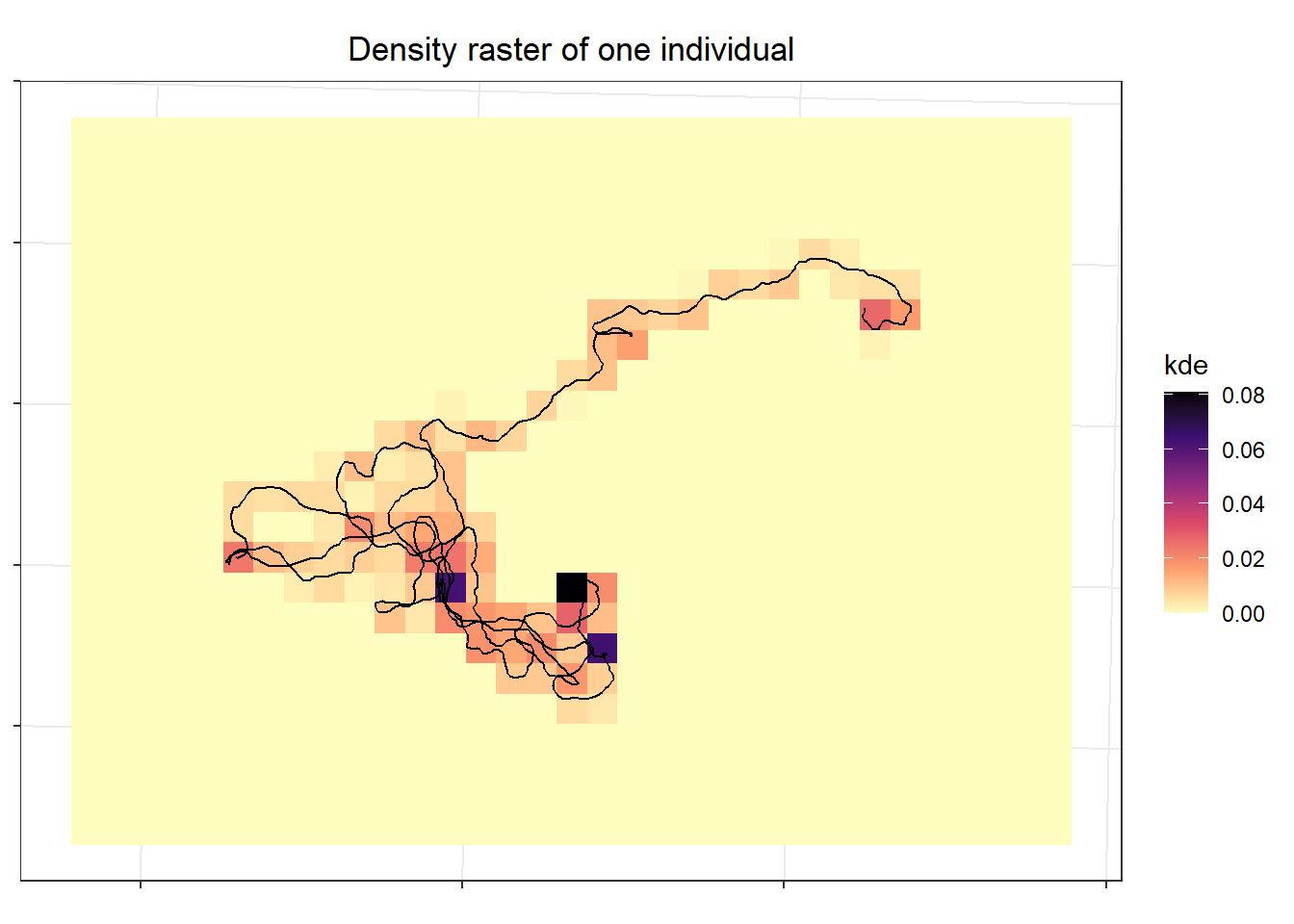
## Exposure risk
For each individual I calculate their utilization distribution based purely on the proportion of points in each cell (density). For real movement data using more accurate estimates of utilization distributions such as kernel density, Brownian bridge movement models, etc. However, those methods are slow.
To figure out how to do this, I first tried it out with just one individual.
```{r}
## which individual (1-100)
who = 1
## kernel density estimate
kde.trial <- terra::rasterize(st_cast(sim.rw.levy[who,], "MULTIPOINT"), riskmap, fun = "length", background = 0)/nsteps

if(sum(values(kde.trial), na.rm=T) != 1){
  stop("the sum of the density should be equal to 1")
}
```
```{r, include=F, eval=FALSE}
### this is resulting in kde map that doesn't align with the track
## need a list of the coordinates for one individual
kde.trial <- sim.rw.levy[1,] %>%
st_coordinates() %>%
as.data.frame
### use mass kde function
kde.trial <- MASS::kde2d(x = kde.trial$X,
y = kde.trial$Y)#,
# n=c(ncol(riskmap),
# nrow(riskmap)))#, lims = ext(riskmap)[1:4])
## make back into rast
kde.trial <- rast(kde.trial$z,
crs = crs(riskmap),
extent = ext(riskmap))
## plot
ggplot() +
stars::geom_stars(data = stars::st_as_stars(kde.trial)) +
scale_fill_viridis_c(option = "D") +
coord_fixed() +
labs(x=NULL, y=NULL, fill = "kde", title = "Density estimate for one individual") +
theme(axis.text = element_blank()) +# since don't care about location
geom_sf(data = sim.rw.levy[1,])
```
To see what that looks like, for the single individual I cropped to just the immediate area that individual used the plot their density estimate.
```{r}
## crop to area where the individual was so not tiny
kde.sm <- terra::crop(kde.trial, st_buffer(sim.rw.levy[who,], 2000))

## similarly crop riskmap to same area
risk.sm <- crop(riskmap, st_buffer(sim.rw.levy[who,], 2000))

## plot traj and kde
ggplot()+
  stars::geom_stars(data = stars::st_as_stars(kde.sm)) +
  scale_fill_viridis_c(option="A", direction = -1) +
  coord_fixed() +
  labs(x=NULL, y=NULL, fill = "kde", title = "Density raster of one individual") +
  theme(axis.text = element_blank()) +# since don't care about location
  geom_sf(data = sim.rw.levy[who,])
```
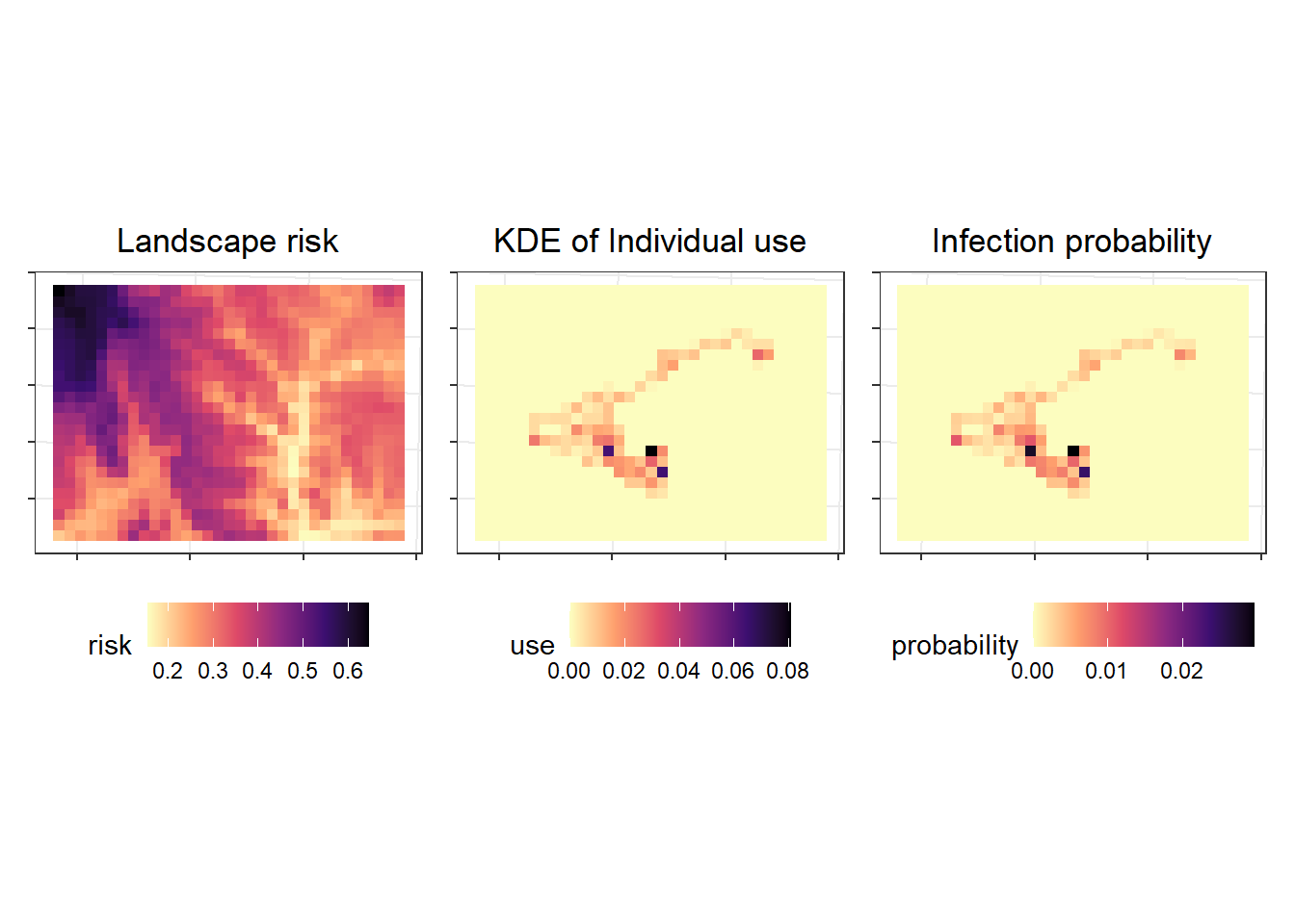
Now I want to calculate the exposure risk for each individual $k$ in each pixel ($i$) as a function of the time they spend in that pixel and the risk of exposure in that pixel.
$$
Exposure_{ki} = kde_i*risk_i
$$
```{r}
## calculate risk
kde.risk <- kde.sm*risk.sm

## plots to demo
p1 <- ggplot()+
  tidyterra::geom_spatraster(data=risk.sm) +
  scale_fill_viridis_c(option="A", direction = -1) +
  labs(title = "Landscape risk", fill = "risk") +
  theme(legend.position = "bottom", axis.text = element_blank(),
        legend.direction = "horizontal")
p2 <- ggplot()+
  tidyterra::geom_spatraster(data=kde.sm) +
  scale_fill_viridis_c(option="A", direction = -1) +
  labs(title = "KDE of Individual use", fill = "use") +
  theme(legend.position = "bottom", axis.text = element_blank(),
        legend.direction = "horizontal")
p3 <- ggplot()+
  tidyterra::geom_spatraster(data=kde.risk) +
  scale_fill_viridis_c(option="A", direction = -1) +
  labs(title = "Infection probability", fill = "probability") +
  theme(legend.position = "bottom", axis.text = element_blank(),
        legend.direction = "horizontal")
p1 + p2 + p3
```
```{r}
#| include: false
#### clean up examples
rm(kde.sm, risk.sm, kde.risk, p1, p2, p3, who)
```
Therefore for each individual $k$ their cumulative 'exposure risk' the sum of all their exposures in pixels, where $i$ is $1:n_{pixels}$: $$
Exposure_k = \sum{kde_i*risk_i}
$$
To calculate the cummulative exposure risk for all individuals, I used a function.
```{r}
#| code-fold: show
## make a function
measure_risk <- function(walker, riskmap, nsteps){

  ## convert from lines to points
  pts <- st_cast(walker, "MULTIPOINT")

  ## dataframe with any attributes (just IDs)
  df <- pts %>% st_drop_geometry() %>% as.data.frame()

  pts <- vect(pts)

  ## for each individual rasterize their points so have sum of points in each pixel
  ## this is not working using the stars::st_rasterize, or the terra::rasterize -- both return one object of all individuals, not an obj per indiv
  ## also tried using apply, lapp, and app with those terra::rasterize
  kde <- c()
  for(i in 1:nrow(pts)){
    kde[[i]] <- terra::rasterize(pts[i,], riskmap, fun = "length", background = 0)/nsteps
  }

  ## multiply time in cell (kde) * cell's risk
  kde.risk <- lapply(kde, function(i) i*riskmap)

  ## sum of values in each layer are individual's risk
  indiv.risk <- lapply(kde.risk, function(i) sum(values(i), na.rm=T))

  df$exp_risk <- unlist(indiv.risk)

  return(df)
}
```
I found the cummulative expsoure risk for each individual using the function.
```{r}
#| echo: false
#| message: false
## calculate individual risk for the brownian (1) and correlated (2)
indiv.risk.rw <- measure_risk(walker = sim.rw.sfc, riskmap = riskmap, nsteps = nsteps)
indiv.risk.levy <- measure_risk(walker = sim.rw.levy, riskmap = riskmap, nsteps = nsteps)
```
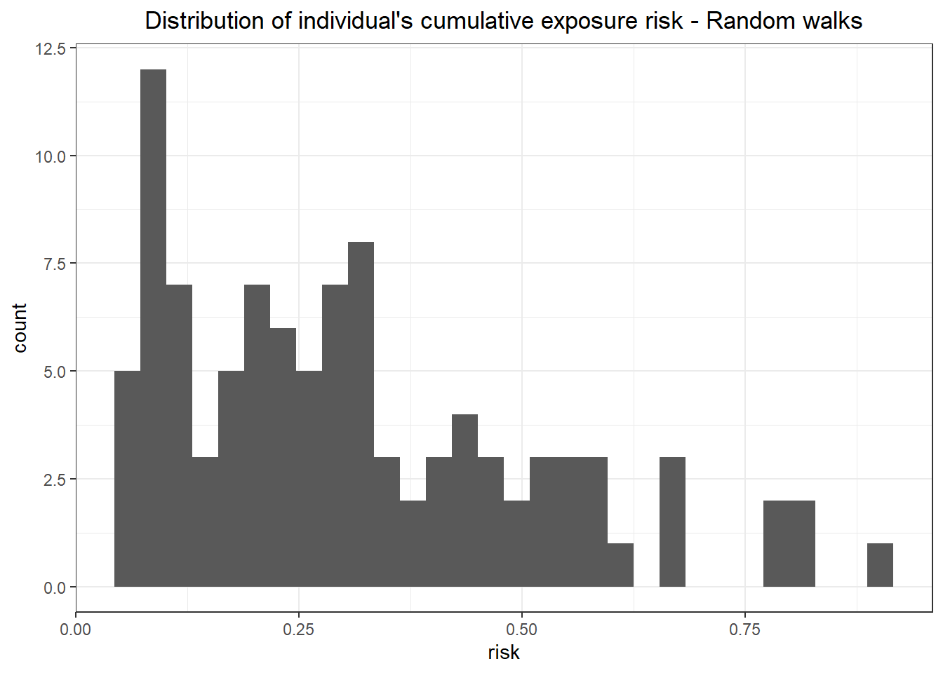
The distribution of values in the random walkers is the range of the map, which is expected.
```{r}
## look at some of the values
# indiv.risk.rw %>% head() %>% knitr::kable(title = "Cummulative exposure risk (`exp_risk`) by individual (`id`)")
indiv.risk.rw %>%
  ggplot()+
  geom_histogram(aes(x = exp_risk)) +
  labs(x = "risk", title = "Distribution of individual's cumulative exposure risk - Random walks")
```
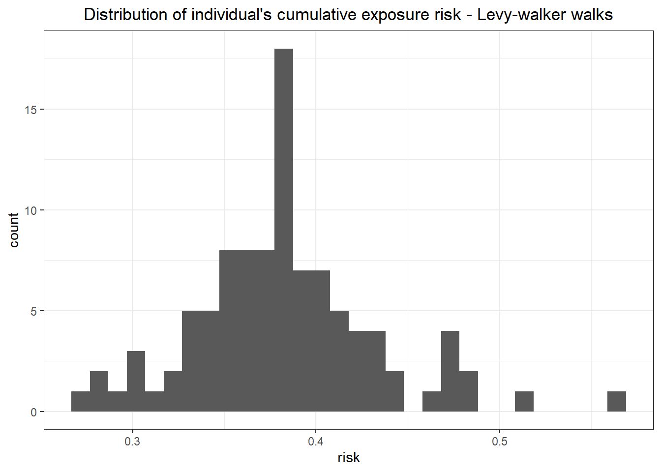
The distribution of values in the correlated walkers is less then the range of the map, which is also expected.
```{r}
# indiv.risk.levy %>% head()
indiv.risk.levy %>%
  ggplot()+
  geom_histogram(aes(x = exp_risk)) +
  labs(x = "risk", title = "Distribution of individual's cumulative exposure risk - Levy-walker walks")
```
## Assisgn susceptibility
Individuals should have variable susceptibility so that not everyone's probability of infection equals their risk sum. This is adding noise to the data. I want to compare the randomly assign susceptibility to a fixed susceptibility for each simulation. The fixed susceptibility is just the average susceptibility of all individuals in that round of the simulation. For this simulation I am assigning susceptibility randomly using a uniform distribution between 0.7 and 0.9. and the fixed susceptibility with the average of the random susceptibility values.
```{r}
#| code-fold: show
## susceptibility is variable between individuals
susceptibility = runif(100, 0.7, 0.9)
mean_suscept = mean(susceptibility)
```
The probability of infection is a product of the individuals exposure risk and susceptibility.
```{r}
#| tbl-cap: Infections in Random Walkers
#| tbl-subcap: ["exposure*susceptibility", "exposure*avg susceptbility"]
#| layout-ncol: 2
## make a dataframe for the outcomes --- random walkers
rw_risk <- cbind(indiv.risk.rw,
                 data.frame( susceptibility = susceptibility)) %>%
  rowwise() %>%
  ## predict infections based on exposure risk
    mutate(infected_es = rbinom(1, 1, exp_risk * susceptibility ), # sum(exp_risk * susceptibility)
           infected_e = rbinom(1, 1, exp_risk * mean_suscept)) # sum(exposure risk) alone

## see how many people infected  = 1
rw_risk %>% count(infected_es) %>% knitr::kable()
rw_risk %>% count(infected_e) %>% knitr::kable()
```
```{r}
#| tbl-cap: Infections in Correlated Walkers
#| tbl-subcap: ["exposure*susceptibility", "exposure*avg susceptbility"]
#| layout-ncol: 2
#|
## make a dataframe for the outcomes --- levy walkers
levy_risk <- cbind(indiv.risk.levy,
                 data.frame( susceptibility = susceptibility)) %>%
  rowwise() %>%
  ## predict infections based on exposure risk
    mutate(infected_es = rbinom(1, 1, exp_risk * susceptibility ), # sum(exp_risk * susceptibility)
           infected_e = rbinom(1, 1, exp_risk * mean_suscept)) # sum(exposure risk) alone

## see how many people infected  = 1
levy_risk %>% count(infected_es) %>% knitr::kable()
levy_risk %>% count(infected_e) %>% knitr::kable()
```
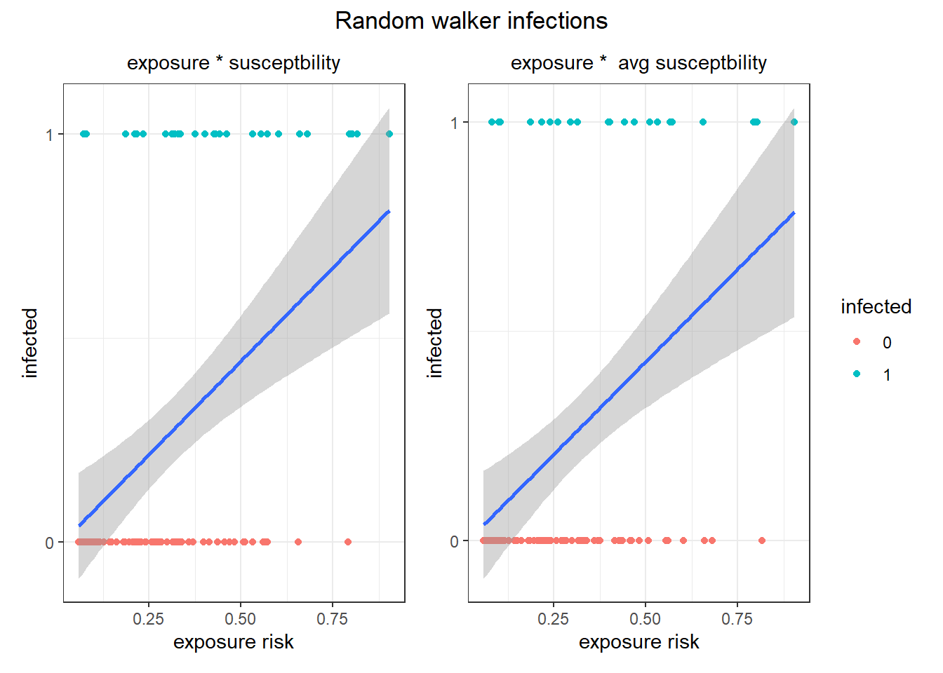
## Results
If the map worked, then exposure risk should predict infection in the random walkers.
```{r}
p1 <- ggplot(rw_risk, aes(x=exp_risk, y = infected_es))+
  geom_point(aes(col=factor(infected_es))) +
  geom_smooth(method="lm") +
  scale_y_continuous(breaks = c(0, 1)) +
  labs(x = "exposure risk", y = "infected", col = "infected", subtitle = "exposure * susceptbility")

p2 <- ggplot(rw_risk, aes(x=exp_risk, y = infected_e))+
  geom_point(aes(col=factor(infected_e))) +
  geom_smooth(method="lm") +
  scale_y_continuous(breaks = c(0, 1)) +
  labs(x = "exposure risk", y = "infected", col = "infected", subtitle = "exposure *  avg susceptbility")
p1 + p2 + plot_layout(guides = "collect") + plot_annotation(title = "Random walker infections")
```
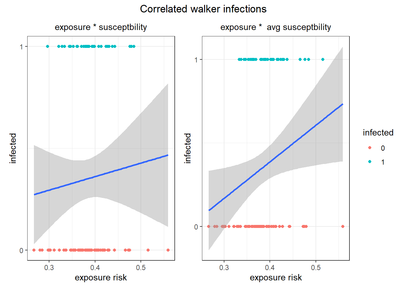
Not great, but the infected individuals do have higher exposure risks. Let's see how it worked for the Levy-walker correlated walkers that covered much more ground.
```{r}
p1 <- ggplot(levy_risk, aes(x=exp_risk, y = infected_es))+
  geom_point(aes(col=factor(infected_es))) +
  geom_smooth(method="lm") +
  scale_y_continuous(breaks = c(0, 1)) +
  labs(x = "exposure risk", y = "infected", col = "infected", subtitle = "exposure * susceptbility")

p2 <- ggplot(levy_risk, aes(x=exp_risk, y = infected_e))+
  geom_point(aes(col=factor(infected_e))) +
  geom_smooth(method="lm") +
  scale_y_continuous(breaks = c(0, 1)) +
  labs(x = "exposure risk", y = "infected", col = "infected", subtitle = "exposure *  avg susceptbility")
p1 + p2 + plot_layout(guides = "collect") + plot_annotation(title = "Correlated walker infections")
```
Compare predictive accuracy between the models
```{r}
pred_acc_fun <- function(x, infected_type){
  x$infected <- x %>% dplyr::select(any_of(infected_type)) %>% pull()

  ## binomial model
  mod <- glm(infected ~ exp_risk, data = x, family = "binomial")
  ## predicted prob of infection
  x$pred_prob <- predict(mod, x, type = "response")
  ## if predicted prob >50 say infected
  x$pred <- 1*(x$pred_prob > .5)
  x$accurate <- 1*x$infected == x$pred
  sum(x$accurate) /nrow(x)

}
```
The accuracy of the infection predictions should be highest in the random walk individuals with fixed susceptibility (exp_risk \* avg susceptibility), followed by those with random susceptibility, then correlated walkers with fixed, then random susceptibility.
```{r}
data.frame(walker = c("Random", "Random", "Correlated", "Correlated"),
           susceptibility = c("Fixed", "Random", "Fixed", "Random"),
           accuracy = c(pred_acc_fun(rw_risk, "infected_e"),
                        pred_acc_fun(rw_risk, "infected_es"),
                        pred_acc_fun(levy_risk, "infected_e"),
                        pred_acc_fun(levy_risk, "infected_es")
                        )) %>%
  knitr::kable(title = "Predictive accuracy of infection probabilities")
```
```{r}
#| include: false
## clean up
rm(levy_risk, indiv.risk.levy, indiv.risk.rw, p1, p2, rw_risk, sim.rw.levy, sim.rw.sfc)
```
# Large Simulation
Ultimately to see how cumulative exposure risk predicts infection in people, the simulation needs to be run many times. To do that everything from the single simulation needs to be in a single function.
```{r}
simulation_fun <- function(n_steps = 1000, n_individuals = 100, susceptibility_range = c(0.7, 0.9),
                           risk_landscape = riskmap, study_area = aoi, landscape_resistance = resistance,
                           random_walker = rand.walker, correlated_walker = levy.walker){

  ## simulate movement
  ### Random (brownian) walks
  ## random starting coordinates
  start_coord <- st_sample(study_area, 100, type = "random")
  start_coord <- st_coordinates(start_coord)

  ## simulate single state walks of 1000 steps
  sim.rw <- list()
  for (i in 1:n_individuals) {
    ## simulate from location i
    tmp <- simulate(random_walker, n_steps,
                    coords = start_coord[i,])
    ## save results to a list
    sim.rw[[i]] <- cbind(tmp[,1], tmp[,2])
  }

  ## make in to sfc lines
  walks.random <- lapply(sim.rw, st_linestring)
  walks.random <- st_sf(id = 1:n_individuals, geometry = walks.random) %>%
    st_set_crs(st_crs(risk_landscape))

  ### Levy-walker (correlated random)
  ## new starting coords in areas of low resistance so don't get stuck
  init = xyFromCell(resistance, sample(which(values(resistance) == 0), 100, replace=T))

  ## simulate
  sim.rw <- list()
  for (i in 1:n_individuals) {
    ## simulate from location i
    tmp <- simulate(correlated_walker, n_steps,
                    resist = raster(resistance),
                    coords = init[i,])
    ## save results to a list
    sim.rw[[i]] <- cbind(tmp[,1], tmp[,2])
  }

  ## make in to sfc lines
  walks.corr <- lapply(sim.rw, st_linestring)
  walks.corr <- st_sf(id = 1:100, geometry = walks.corr) %>%
    st_set_crs(st_crs(risk_landscape))

  ## Calculate cumulative exposure risk/individual
  ### random walkers
  indiv.risk.random <- measure_risk(walker = walks.random, riskmap = risk_landscape, nsteps = n_steps)
  ### correlated random walkers
  indiv.risk.corr <- measure_risk(walker = walks.corr, riskmap = risk_landscape, nsteps = n_steps)

  ## assign susceptibility
  susceptibility = runif(100, susceptibility_range[1], susceptibility_range[2])
  mean_suscept = mean(susceptibility)

  ## determine infections
  ## make a dataframe for the outcomes --- random walkers
  indiv.risk.random <- cbind(indiv.risk.random,
                   data.frame( susceptibility = susceptibility)) %>%
    rowwise() %>%
    ## predict infections based on exposure risk
    mutate(infected_es = rbinom(1, 1, exp_risk * susceptibility ), # sum(exp_risk * susceptibility)
           infected_e = rbinom(1, 1, exp_risk * mean_suscept)) # sum(exposure risk) alone

  ## make a dataframe for the outcomes --- levy walkers
  indiv.risk.corr <- cbind(indiv.risk.corr,
                     data.frame( susceptibility = susceptibility)) %>%
    rowwise() %>%
    ## predict infections based on exposure risk
    mutate(infected_es = rbinom(1, 1, exp_risk * susceptibility ), # sum(exp_risk * susceptibility)
           infected_e = rbinom(1, 1, exp_risk * mean_suscept)) # sum(exposure risk) alone


  ## output predictive accuracy
  data.frame(walker = c("Random", "Random", "Correlated", "Correlated"),
           susceptibility = c("Fixed", "Random", "Fixed", "Random"),
           accuracy = c(pred_acc_fun(indiv.risk.random, "infected_e"),
                        pred_acc_fun(indiv.risk.random, "infected_es"),
                        pred_acc_fun(indiv.risk.corr, "infected_e"),
                        pred_acc_fun(indiv.risk.corr, "infected_es")
                        ))
}
```
Check that the function works when run one time. By default the simulation uses the riskmap, aoi, resistance raster, and random and levy walker walks set up previously. The default number of steps in each walk is 1000, for 100 individuals, with susceptibility \[0.7, 0.9\] as used previously.
```{r}
## check it works running one time
simulation_fun() %>% knitr::kable(title = "Results of one simulation using the function")
```
Then run the function 100 times.
```{r}
## fun the function many times
lg_sim <- replicate(100, simulation_fun(), simplify = F)

## make the output into one large dataframe
lg_sim <- bind_rows(lg_sim)
```
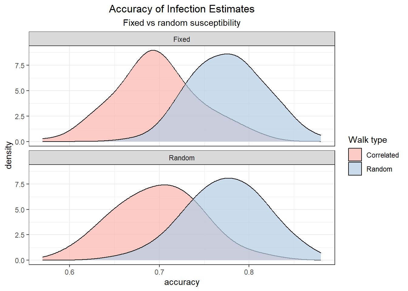
The distributions of the accuracy of models that use cumulative exposure to predict infection show that as expected random walkers infections are predicted with higher accuracy, and that the effect of variable susceptibility to infection in each individual lower the accuracy of correlated walks more than random walks.
```{r}
## plot the distribution of predictive values between the fix susceptibility random and correlated walks
lg_sim %>%
  ggplot(aes(x=accuracy, fill=walker)) +
  geom_density(adjust =1.5, alpha = 0.7) +
  scale_fill_brewer(palette = "Pastel1")+
  facet_wrap(~susceptibility, ncol=1)+
  labs(title = "Accuracy of Infection Estimates",
       subtitle = "Fixed vs random susceptibility",
       fill = "Walk type")
```
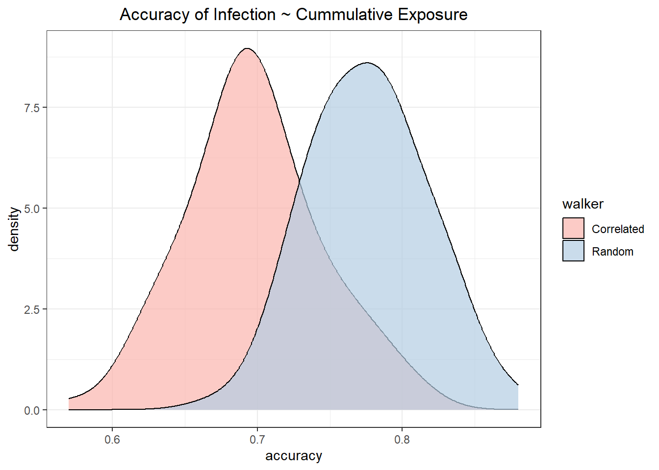
The predictive accuracy of the simulations that used the fixed susceptibility values for all individuals (infection is only related to cumulative exposure risk) is significantly higher in random walkers then correlated walkers.
```{r}
## plot the distribution of predictive values between the fix susceptibility random and correlated walks
lg_sim %>%
  filter(susceptibility == "Fixed") %>%
  ggplot(aes(x=accuracy, fill=walker)) +
  geom_density(adjust =1.5, alpha = 0.7) +
  scale_fill_brewer(palette = "Pastel1")+
  labs(title = "Accuracy of Infection ~ Cummulative Exposure")
## test if significantly different
lg_sim %>%
  filter(susceptibility == "Fixed") %>%
  t.test(accuracy ~ walker, data = ., var.equal = TRUE)
```
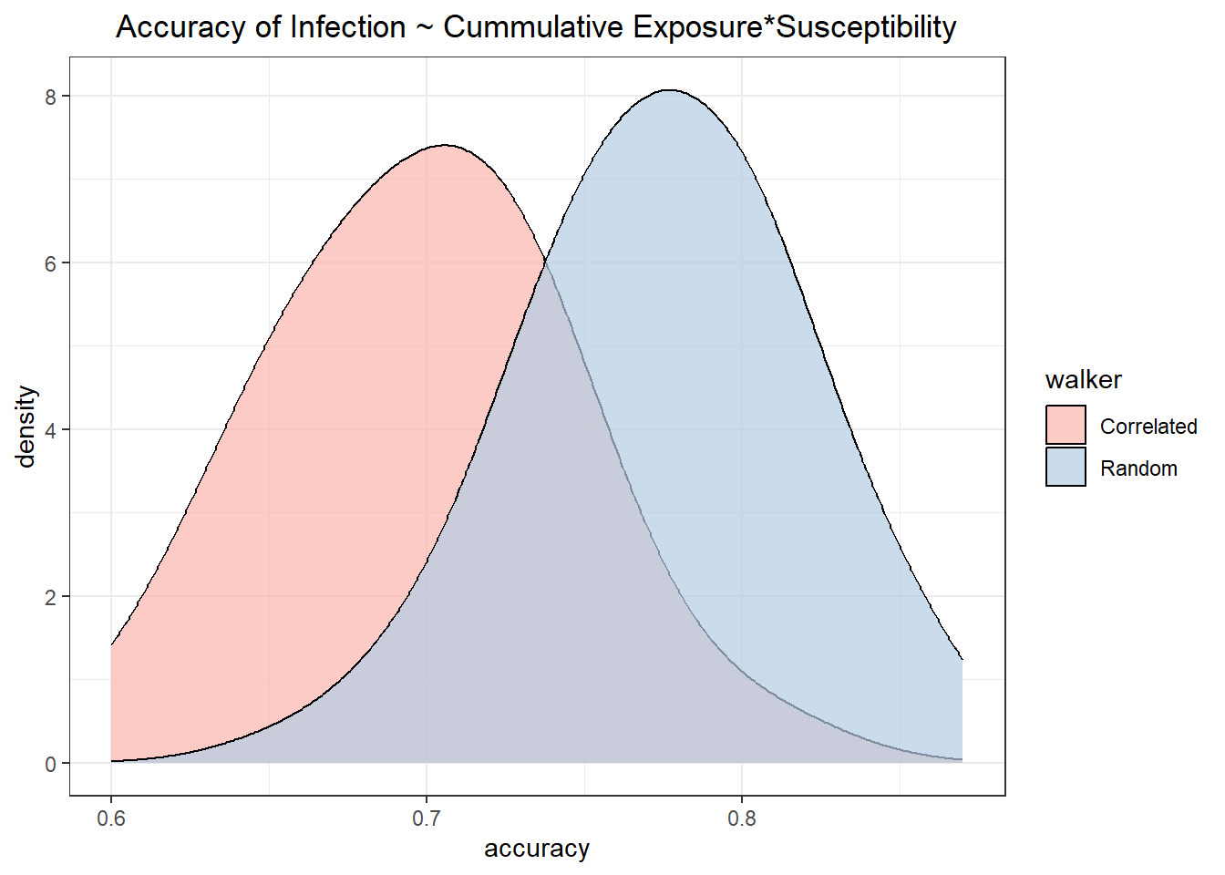
The same effect is seen in the randomly assigned individual susceptibility random and correlated walkers.
```{r}
## plot the distributions of predictive values between the variable susceptibility random and correlated walks
lg_sim %>%
  filter(susceptibility == "Random") %>%
  ggplot(aes(x=accuracy, fill=walker)) +
  geom_density(adjust =1.5, alpha = 0.7) +
  scale_fill_brewer(palette = "Pastel1")+
  labs(title = "Accuracy of Infection ~ Cummulative Exposure*Susceptibility")
## test if significantly different
lg_sim %>%
  filter(susceptibility == "Random") %>%
  t.test(accuracy ~ walker, data = ., var.equal = TRUE)
```
# Conclusion
To wrap up the simulation showed that predicting individual infection probability as defined by their cumulative exposure risk, is influence by the amount of noise in that dataset such as we would expect to observe due to variability in individual's susceptibility to infection. Future directions include rerunning this simulation over different susceptibility windows and using predictors that correlate with, but are not the 'real' risk landscape.
# References